Interest Rate Parity

Spot FX and CFDs, Currency Concepts / PhillipCapital DIFC Research Team

Interest Rate Parity Understanding Interest Rate Parity: A Guide to Currency Concepts The foreign exchange market is driven by an invisible web of economic forces. Among the most powerful of these forces are interest rates. For investors navigating global markets, understanding how central bank policies influence currency valuation is crucial. This is where the concept of Interest Rate Parity comes into play. It acts as the mathematical bridge connecting the interest rates of two distinct nations with the exchange rate of their currencies. Let’s explore the mechanics of this fundamental economic theory and how it impacts global trading strategies. Table of Contents What is Interest Rate Parity (IRP)? How Does Interest Rate Parity Work in Currency Markets? What is the Difference Between Covered and Uncovered Interest Rate Parity? Why is Interest Rate Parity Important for Investors? What Happens When Interest Rate Parity is Broken? Conclusion & Key Takeaways What is Interest Rate Parity (IRP)? Interest Rate Parity (IRP) is a foundational economic theory used in the foreign exchange market. At its core, IRP states that the difference in interest rates between two countries should equal the expected change in exchange rates between their respective currencies. In simpler terms, if you invest your money in a country with higher interest rates, you should not be able to make a guaranteed, risk-free profit compared to investing in a country with lower interest rates. Why? Because the currency of the country with the higher interest rate is expected to depreciate against the currency with the lower interest rate over time. This concept ensures that global markets remain in balance. Without this parity, investors could easily borrow money in a country with low interest rates, exchange it, and invest it in a country with high interest rates to make a guaranteed, risk-free profit. To fully grasp this dynamic, it is helpful to first understand the mechanics of the base currency and quote currency, as these components dictate exactly how exchange rates are quoted, calculated, and impacted by shifting rates. How Does Interest Rate Parity Work in Currency Markets? To understand how Interest Rate Parity works practically, imagine a scenario involving two major economies. Let’s say Country A has an annual interest rate of 5%, while Country B has an interest rate of 2%. Under the rules of Interest Rate Parity, the 3% difference in interest rates will be offset by the currency market. Specifically, Country A’s currency is expected to weaken by 3% against Country B’s currency over the course of the year. This depreciation neutralizes the advantage of the higher interest yield. When you look at the major currency pairs traded heavily on global exchanges, their forward pricing relies strictly on these interest rate differentials. If the exchange rate did not automatically adjust to reflect the difference in interest rates, institutional investors would rapidly exploit the gap—a process known as arbitrage—until the market corrected itself and parity was restored. Ready to Trade Global Currency Pairs? Apply your understanding of interest rates to the real-world forex markets. Explore Forex Trading What is the Difference Between Covered and Uncovered Interest Rate Parity? Interest Rate Parity is generally divided into two distinct categories: Covered and Uncovered. Understanding the difference between the two is vital for proper financial risk management. Covered Interest Rate Parity (CIRP) Covered Interest Rate Parity occurs when forward exchange rates (agreed-upon rates for future currency exchanges) perfectly offset the difference in interest rates between two countries. In this scenario, an investor uses a forward contract to “cover” or hedge against the risk of the exchange rate fluctuating. Because the future exchange rate is locked in from day one, the investor completely eliminates currency risk. The mathematical reality of CIRP means that taking advantage of higher interest rates abroad, while hedging with a forward contract, will yield the exact same return as investing safely domestically. Uncovered Interest Rate Parity (UIRP) Uncovered Interest Rate Parity operates on the same basic principle but without the safety net of a forward contract. Here, the investor does not “cover” their position. Instead, they rely purely on the expected future spot exchange rate. UIRP assumes that the currency with the higher interest rate will naturally depreciate by the exact amount of the interest rate differential. Because there is no forward contract locking in the price, UIRP carries significant exchange rate risk. If the currency market behaves unexpectedly, the investor could face substantial losses. Why is Interest Rate Parity Important for Investors? Interest Rate Parity is not just an academic theory; it is a highly practical tool used by global investors to evaluate currency valuations and manage portfolio risk. Firstly, it helps institutional traders identify potential mispricings in the market. If Covered Interest Rate Parity is temporarily broken, large financial institutions can execute risk-free arbitrage strategies, instantly buying and selling currencies across borders to capture a guaranteed profit before the market corrects itself. Secondly, understanding these interest rate differentials is crucial for investors executing carry trades. A carry trade involves borrowing a currency with a low interest rate to fund the purchase of a currency with a high interest rate. While major pairs are often used for this, traders frequently look toward minor and exotic currency pairs to find the largest, most lucrative interest rate gaps. However, traders must remember that according to Uncovered Interest Rate Parity, the high-yielding currency is theoretically expected to depreciate, which can quickly wipe out the interest earned if the market moves aggressively against them. Discover High-Yield Opportunities Explore exotic and minor currency pairs to leverage global interest rate differentials Learn About Exotic Pairs What Happens When Interest Rate Parity is Broken? In highly liquid, modern financial markets, Covered Interest Rate Parity holds true almost all the time. When it is momentarily broken, automated trading algorithms immediately execute massive volumes of arbitrage trades, snapping the market back into balance within fractions of a second. However, true parity can sometimes be hindered by real-world friction. Capital controls, varying international tax laws, and sudden drops in

Interest Rate Parity Read More »

Initial vs. Maintenance Margin

Uncategorized, Educational Blogs, Exchange Traded Derivatives, Futures Contracts / PhillipCapital DIFC Research Team

Initial vs. Maintenance Margin Understanding Initial and Maintenance Margins: A Comprehensive Guide In the world of professional trading, leverage is a powerful tool that allows investors to increase their market exposure. However, to use leverage effectively, one must understand the “collateral” rules set by exchanges and brokers. These rules are governed by two primary concepts: Initial Margin and Maintenance Margin. Whether you are trading equities, futures, or currencies, grasping these terms is essential for protecting your capital and avoiding the dreaded “margin call.” This guide breaks down everything you need to know in a clear, professional manner. Table of Contents What is the fundamental difference between Initial and Maintenance Margin? How does Initial Margin work when opening a new position? Why is Maintenance Margin critical for risk management? What happens if your account balance falls below the Maintenance Margin? How can traders effectively manage margin requirements? Conclusion & Key Takeaways What is the fundamental difference between Initial and Maintenance Margin? To trade on leverage, you aren’t required to pay the full value of an asset upfront. Instead, you provide a portion of the value as a “good faith deposit.” The Initial Margin is the percentage of the purchase price that an investor must pay for with their own cash when establishing a position. Think of it as the entry requirement. On the other hand, the Maintenance Margin is the minimum amount of equity that must remain in the account as long as the position is open. While the initial margin is about starting a trade, the maintenance margin is about keeping it. If the market moves against you and your account equity drops, the maintenance level acts as a floor to ensure you have enough funds to cover potential losses. This is a core part of the trading products we offer, where margin requirements vary by asset class. How does Initial Margin work when opening a new position? When you decide to enter a trade—for example, in the global futures and options market—the exchange sets a specific dollar amount or percentage required to hold that contract. This is your Initial Margin. For instance, if you wish to buy $100,000 worth of an asset and the initial margin requirement is 10%, you must have at least $10,000 in your account. This allows you to control a large position with a relatively small amount of capital. It is important to note that these requirements can change based on market volatility; during periods of high uncertainty, brokers may increase these rates to protect both the firm and the client. Why is Maintenance Margin critical for risk management? Once your trade is live, the value of your account fluctuates every second. The Maintenance Margin ensures that you always have a “buffer.” Regulatory bodies usually set this lower than the initial margin—often around 25% to 30% of the total value of the securities. The reason this is so critical is that it protects the integrity of the market. By ensuring traders maintain a minimum equity level, it prevents a scenario where a trader owes more than they have in their account. For those trading CFDs or other fast-moving assets, monitoring these levels across different positions is vital to ensure that a drop in one asset doesn’t trigger liquidations across your entire portfolio. View Investment Solutions Explore our wide range of trading products. View Products What happens if your account balance falls below the Maintenance Margin? If the market moves against your position and your account equity dips below the maintenance threshold, you will receive a Margin Call. This is a formal notice from your broker requesting that you deposit more funds or close out positions to bring the account back up to the required level. If a trader fails to meet the margin call promptly, the broker has the right to close (liquidate) the positions at the current market price to prevent further losses. This is why many experienced traders check our daily market updates regularly to stay ahead of price swings that could impact their margin health. How can traders effectively manage margin requirements? Managing margin is less about the math and more about discipline. Here are three professional strategies: Maintain Excess Liquidity: Never use 100% of your available margin. Keeping a “cash cushion” allows your positions to breathe during normal market fluctuations. Monitor Volatility: In volatile markets, margin requirements can increase suddenly. Staying updated on Indian equity markets or global trends can help you anticipate these changes. Use Stop-Loss Orders: By setting a price at which your trade automatically closes, you can ensure your equity never drops near the maintenance margin level. By staying informed and using the resources provided by PhillipCapital, investors can set alerts and monitor their margin utilization in real-time. Conclusion & Key Takeaways Understanding the distinction between initial and maintenance margins is a non-negotiable skill for any trader using leverage. While the initial margin gets you into the market, the maintenance margin keeps you there safely. Key Takeaways: Initial Margin: The “entry fee” or the upfront capital required to open a leveraged position. Maintenance Margin: The minimum equity required to keep the position active. Margin Calls: Triggered when equity falls below maintenance levels, requiring immediate action. Risk Control: Best achieved by keeping extra capital and staying educated on market movements. Partner With PhillipCapital Open an account with a trusted, regulated broker. Open Live Account Frequently Asked Questions (FAQs) How do I actually know if a stock is “high quality”? Look for three primary indicators: consistent profitability over several years, low levels of debt compared to cash reserves, and a strong competitive advantage (like a powerful brand or unique technology). If a company can easily survive a tough economic environment without needing to borrow heavily, it is generally considered a high-quality business. Are quality stocks the same as dividend stocks? Not always. While many high-quality companies pay reliable dividends due to their strong cash flow, others choose to reinvest that cash back into the business to fuel further expansion.

Initial vs. Maintenance Margin Read More »

Currency Carry Trade

Educational Blogs, Currency Concepts, Spot FX and CFDs / PhillipCapital DIFC Research Team

Currency Carry Trade Unlocking Global Yields: The Definitive Guide to the Currency Carry Trade Table of Contents Introduction What is a Currency Carry Trade and How Does It Work? Which Currencies Are Most Commonly Used in Carry Trades? How Does Leverage Impact the Returns of a Carry Trade? What Are the Primary Risks Associated with the Currency Carry Trade Strategy? How Do Central Bank Policies and Interest Rates Influence Carry Trades? Can Retail Investors Effectively Execute a Currency Carry Trade? Conclusion Introduction In the dynamic landscape of global capital markets, sophisticated investors continuously seek strategies that generate yield independent of traditional equity market rallies. Operating from strategic financial hubs like Dubai, which bridges East and West, provides a unique vantage point to capitalize on macroeconomic divergences across the globe. One of the most historically prominent strategies for capturing these macroeconomic shifts is the currency carry trade. By leveraging the differences in borrowing costs between nations, investors can essentially get paid for holding a position over time. However, this strategy is not without its complexities. Successfully navigating the carry trade requires a deep understanding of monetary policy, currency valuations, and rigorous risk management. This guide explores the mechanics, opportunities, and inherent risks of deploying this strategy in today’s volatile markets. What is a Currency Carry Trade and How Does It Work? At its core, a currency carry trade is an investment strategy where a trader borrows a currency from a country with a low interest rate (the funding currency) to purchase a currency from a country with a high interest rate (the target or asset currency). The primary objective is to capture the “yield differential” or the “carry”—the difference between the interest earned on the high-yielding currency and the interest paid on the borrowed low-yielding currency. Mechanically, when you execute a trade in the foreign exchange market, you are simultaneously buying one currency and selling another. If you buy a currency pair where the base currency has a higher interest rate than the quote currency, your broker will typically credit your account with a daily “rollover” or “swap” fee for every day you hold the position open past the daily market close. Conversely, if the situation is reversed, you would pay this fee. The strategy assumes that the exchange rate between the two currencies will either remain stable or appreciate in favor of the high-yielding currency, allowing the trader to pocket the interest difference without suffering capital losses from currency depreciation. Which Currencies Are Most Commonly Used in Carry Trades? The selection of currencies is the foundational building block of a successful carry trade. Historically, the most effective trades pair stable, low-inflation economies with those experiencing robust growth and higher borrowing costs. The Funding Currencies: The Japanese Yen (JPY) and the Swiss Franc (CHF) have historically been the premier funding currencies. For decades, the Bank of Japan maintained zero or even negative interest rates to combat deflation, making the Yen exceptionally cheap to borrow. The Target Currencies: Historically, the Australian Dollar (AUD) and New Zealand Dollar (NZD) served as prime target currencies due to their commodities-backed economies and higher domestic rates. Emerging Markets: Modern traders often look toward exotic currency pairs to find larger yield spreads. Currencies like the South African Rand (ZAR) or the Mexican Peso (MXN) often boast significantly higher interest rates to attract foreign capital, though they come with elevated volatility. Expand Your Forex Strategy Capitalize on global interest rate differentials with access to a wide range of global currencies. Explore Currency Pairs How Does Leverage Impact the Returns of a Carry Trade? A 3% or 4% annual interest rate differential might seem insignificant to an aggressive investor. However, the true power—and danger—of the carry trade lies in the use of leverage. Because currencies typically experience much lower daily percentage movements compared to equities, brokers offer significant leverage on Spot FX trading accounts. If a trader identifies a pair with a 4% yield differential and applies 10:1 leverage, the annualized yield on the invested margin jumps to 40% (excluding broker fees and spread costs). However, leverage is a double-edged sword. While it exponentially magnifies the yield, it equally magnifies the exposure to exchange rate fluctuations. A minor adverse movement in the currency pair can quickly wipe out months of accumulated interest and lead to a margin call. What Are the Primary Risks Associated with the Currency Carry Trade Strategy? The allure of steady daily income often masks the severe risks inherent in this strategy. The carry trade is famously described as “picking up pennies in front of a steamroller” because the gains are slow and steady, but the losses can be sudden and catastrophic. Exchange Rate Risk: This is the most significant threat. If the high-yielding currency depreciates against the funding currency by an amount greater than the earned interest, the trade results in a net loss. Unwinding Risk: Carry trades are highly sensitive to global risk sentiment. During periods of geopolitical shock or financial panic (often referred to as “risk-off” environments), investors rush to safe-haven currencies (like the JPY or USD) and dump high-yielding, riskier assets. This mass exodus causes a rapid appreciation of the funding currency, leading to sharp, devastating losses for carry traders. Interest Rate Shifts: Understanding exchange rates requires monitoring central banks. If the funding country unexpectedly raises interest rates or the target country lowers them, the yield differential narrows, reducing profitability and often triggering an adverse currency valuation swing. Trade with Confidence in the DIFC Access powerful platforms, deep liquidity, and a comprehensive suite of Spot FX and CFD instruments. Discover Trading Products How Do Central Bank Policies and Interest Rates Influence Carry Trades? Central banks are the architects of the carry trade environment. Their monetary policy decisions dictate the “cost of money,” which in turn drives global capital flows. When the US Federal Reserve embarks on a rate-hiking cycle to combat inflation, the US Dollar often transitions from a potential funding currency into a target currency, drawing capital away from emerging

Currency Carry Trade Read More »

Contango & Backwardation Explained

Futures Contracts, Educational Blogs, Exchange Traded Derivatives / PhillipCapital DIFC Research Team

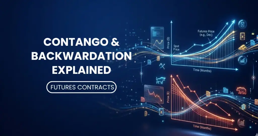
Contango and Backwardation Explained Contango and Backwardation Explained: Navigating Futures Market Curves In the intricate landscape of global capital markets, institutional and sophisticated retail investors rely heavily on derivative instruments to hedge risks, discover prices, and deploy capital efficiently. Among the most critical concepts for anyone trading in these markets are contango and backwardation. These terms describe the shape of the forward curve—the relationship between the current spot price of an asset and its price for future delivery dates. Correctly interpreting whether a market is in contango or backwardation offers profound insights into global supply and demand dynamics, carrying costs, and market sentiment. This comprehensive guide delves into the mechanics of these market states, exploring what drives them and how professional traders navigate their complexities to optimize portfolio performance. Table of Contents What is the Forward Curve in Futures Trading? What Does Contango Mean in Financial Markets? What Causes a Market to Enter Backwardation? How Do Cost of Carry and Yield Impact Contango and Backwardation? How Can Investors Utilize Contango and Backwardation Strategies? What is the Convergence of Spot and Futures Prices at Expiration? Conclusion What is the Forward Curve in Futures Trading? The forward curve is a graphical representation that plots the prices of futures contracts against their respective expiration dates. Rather than looking at a single price point for an asset like crude oil or a stock index, the forward curve provides a multi-dimensional view of how the market values that asset over time. On the x-axis, you have the maturity timeline (ranging from the nearest expiration date to several months or years into the future), while the y-axis represents the contract price. For professional investors, the shape of this curve is a vital diagnostic tool. It rarely forms a perfectly flat line. Instead, it slopes either upward or downward depending on the aggregate expectations of market participants, prevailing interest rates, and the fundamental supply and demand mechanics of the underlying asset. By analyzing the slope of the forward curve, traders can deduce the market’s implied forecast for future price environments and measure the actual costs associated with holding physical or financial assets over time. What Does Contango Mean in Financial Markets? Contango is widely considered the normal, or standard, state of the futures market. A market is in contango when the futures price of an asset is higher than its current spot price, creating an upward-sloping forward curve. As you look further into the future on the expiration timeline, the contracts become progressively more expensive. This premium on future delivery is not arbitrary. It is heavily driven by the mathematical realities of time-valued money and logistical expenses. When an investor purchases a physical asset today, they incur immediate holding costs, such as warehousing fees, insurance premiums, and the opportunity cost of tying up capital (the risk-free interest rate). Therefore, understanding the relationship between the spot price vs futures price is essential. Buyers in the futures market are willing to pay a premium to lock in a price today while shifting the burden of storing and insuring the asset onto the seller until the future delivery date arrives. In a contango environment, the market is adequately supplied in the short term, and the price curve cleanly reflects the compounded “cost of carry.” Ready to Access Global Futures Markets? Trade international commodities, equities, and FX through a fully regulated platform Explore Futures & Options What Causes a Market to Enter Backwardation? Backwardation is the inverse of contango and is generally considered a rarer, structurally stressed market state. A market falls into backwardation when the futures price is lower than the current spot price, resulting in a downward-sloping forward curve. In this scenario, market participants are paying a heavy premium for immediate possession of the asset rather than waiting for future delivery. This phenomenon is almost exclusively driven by an immediate, urgent imbalance in supply and demand. Severe supply chain disruptions, unexpected geopolitical shocks, or extreme weather events can trigger critical shortages of physical commodities. For example, if a global crisis threatens oil production, refineries cannot wait six months for a futures contract to settle; they need the physical oil immediately to keep operations running. This desperation drives the spot price drastically higher than the deferred futures contracts. Actively calculating the forward-looking basis in futures trading allows investors to detect these supply squeezes early, enabling them to adjust their risk exposure ahead of major macroeconomic adjustments. How Do Cost of Carry and Yield Impact Contango and Backwardation? The concepts of contango and backwardation are fundamentally anchored in two opposing forces: the “cost of carry” and the “convenience yield.” Cost of carry encompasses the explicit expenses required to hold a physical or financial asset. For commodities like gold or wheat, this includes storage space, transit insurance, and financing rates. For financial derivatives, such as equity indices, it primarily involves the prevailing interest rates used to finance the position. These elements form the core of futures fundamentals, dictating how premiums are calculated across different time horizons. When the cost of carry is the dominant force, the market naturally slopes into contango. Conversely, the convenience yield represents the non-financial, operational benefit of physically holding an asset right now. If a manufacturer holds physical copper inventory during a severe supply drought, the convenience yield of keeping their production line open far outweighs the storage costs. When the perceived convenience yield spikes and eclipses the cost of carry, the market is aggressively pushed into backwardation. Additionally, in financial futures, high dividend payouts from underlying stocks can artificially push the curve into backwardation, as futures holders do not receive dividend payments prior to expiration. Master Advanced Derivative Strategies Speak with our institutional trading desk to optimize your portfolio using global derivatives. Contact Our Desk How Can Investors Utilize Contango and Backwardation Strategies? Understanding the shape of the forward curve is paramount for executing long-term trading strategies, particularly those involving the rolling of contracts. When a trader wants to maintain a continuous position in the

Contango & Backwardation Explained Read More »

Magic Formula (Greenblatt’s Strategy)

Trading Strategies, Educational Blogs / PhillipCapital DIFC Research Team

Magic Formula Investing A Guide to Greenblatt’s Systematic Strategy Introduction In the complex ecosystem of global equity markets, identifying sustainable value can often feel overwhelming. Investors are constantly bombarded with macroeconomic noise, speculative trends, and shifting market sentiment. To cut through this volatility, rigorous quantitative frameworks have been developed by leading institutional investors. One of the most renowned is Joel Greenblatt’s Magic Formula—a systematic strategy that ranks stocks by high earnings yield and high return on capital, then buys a basket of the top-ranked stocks. Developed by the founder of Gotham Capital, it is a quantitative value approach designed to find good quality businesses at good prices. By relying strictly on financial mathematics rather than human emotion, the strategy provides a disciplined roadmap for capital allocation. Table of Contents What Is Joel Greenblatt’s Magic Formula Strategy? How Does the Magic Formula Rank Stocks? Why Are Earnings Yield and Return on Capital the Key Metrics? What Are the Advantages of This Quantitative Value Approach? Are There Any Limitations or Risks to the Magic Formula? Conclusion What Is Joel Greenblatt’s Magic Formula Strategy? The Magic Formula is a strictly rules-based value investing framework popularized by hedge fund manager Joel Greenblatt. At its core, the strategy attempts to mathematically codify the legendary investment philosophy of Warren Buffett: buying wonderful companies at fair prices. Instead of relying on subjective forecasts or qualitative business analysis, the formula strips away human bias by focusing entirely on historical financial data. It screens a broad universe of publicly traded companies and ranks them based on two distinct factors: the “cheapness” of the stock (Earnings Yield) and the “quality” of the underlying business (Return on Capital). By combining these two rankings, the strategy identifies a condensed list of companies that offer the optimal intersection of low valuation and high operational efficiency. Before applying advanced quantitative methods to your portfolio, it is imperative to have a solid introduction to stock markets and an understanding of how deliverable equities function within a global framework. The Magic Formula assumes the investor has the capacity to directly purchase and hold actual shares, allowing the underlying business fundamentals to reflect in the stock price over time. How Does the Magic Formula Rank Stocks? The mechanical execution of the strategy is what makes it “systematic.” The ranking process follows a strict, repeatable methodology: Establish a Market Cap Threshold: The strategy begins by defining a universe of investable stocks, typically excluding micro-caps by setting a minimum market capitalization (e.g., $100 million or higher) to ensure adequate market liquidity. Exclude Specific Sectors: Financial institutions (banks, insurance companies) and utility companies are removed from the screening process. Their unique capital structures and heavy regulatory environments make the standard formula metrics less relevant. Calculate Earnings Yield: Every remaining company is ranked by its Earnings Yield, from highest (cheapest) to lowest (most expensive). Calculate Return on Capital: The same companies are then ranked by their Return on Capital (ROC), from highest (most efficient) to lowest (least efficient). Combine the Rankings: The two rank numbers for each company are added together. A company that ranks 15th in Earnings Yield and 10th in ROC would have a combined score of 25. Construct the Basket: The strategy buys a diversified basket of the 20 to 30 companies with the lowest combined scores. These positions are typically held for one year before the portfolio is completely re-evaluated and rebalanced. Access Global Markets with Deliverable Equities Execute value strategies confidently with direct access to US markets. Invest in US Stocks & ETFs Why Are Earnings Yield and Return on Capital the Key Metrics? To understand the power of the strategy, investors must look closely at the specific formulas Greenblatt utilizes, which differ slightly from conventional Wall Street metrics. Earnings Yield (EBIT / Enterprise Value): Traditional investors often use the Price-to-Earnings (P/E) ratio to gauge value. The Magic Formula improves upon this by using Earnings Before Interest and Taxes (EBIT) divided by Enterprise Value (EV). Enterprise Value is a more accurate representation of a company’s price tag because it factors in both the company’s debt and its cash reserves. By using EBIT, the formula evaluates the raw operating profitability of the business before the distortions of varying corporate tax rates and debt interest levels. In short, this metric answers the question: How much operating profit am I getting for the total price of buying the entire business? Return on Capital (EBIT / Net Working Capital + Net Fixed Assets): While traditional Return on Equity (ROE) can be artificially inflated by excessive debt, Greenblatt’s Return on Capital (ROC) measures how effectively a company utilizes its tangible operational assets to generate profit. By dividing EBIT by the sum of net working capital and net fixed assets, the formula isolates the core economic engine of the company. A high ROC indicates a company with a strong competitive advantage, capable of growing its operations without requiring massive external capital injections. Relying solely on surface-level ratios can sometimes lead to poor allocation; therefore, confirming these quantitative signals with a thorough intrinsic value calculation ensures you are deeply analyzing the cash flow generation behind the metrics. What Are the Advantages of This Quantitative Value Approach? The primary advantage of the Magic Formula is its elimination of behavioral finance errors. Human investors are notoriously prone to panic during market corrections and greed during euphoric rallies. By adhering to a systematic, mechanical ranking system, investors are forced to buy out-of-favor companies that possess fundamentally sound operations. Additionally, the strategy enforces portfolio diversification by requiring the purchase of a basket of 20 to 30 stocks. This mitigates single-stock risk, ensuring that a single corporate failure does not devastate the overall capital base. The strategy is also time-efficient; rather than spending hundreds of hours reading subjective analyst reports, the data-driven screen provides a targeted list of high-probability investment candidates. Are There Any Limitations or Risks to the Magic Formula? No quantitative strategy is flawless, and the Magic Formula has distinct challenges. The most prominent risk

Magic Formula (Greenblatt’s Strategy) Read More »

Zero Capital Protection

Structured Products, Educational Blogs, Types of Structured Products / PhillipCapital DIFC Research Team

Zero Capital Protection Understanding Zero Capital Protection: Risks, Rewards, and Investment Strategies Table of Contents Introduction What exactly does “zero capital protection” mean in financial markets? How does a zero capital protection strategy differ from fully protected investments? Why would an investor intentionally choose a product with no capital protection? What are the primary risks associated with zero capital protection structures? Which specific types of structured notes feature zero capital protection? How does this strategy align with a sophisticated wealth management portfolio? Conclusion Introduction In the sophisticated ecosystem of global financial markets, investors are constantly navigating the delicate balance between security and potential returns. While many conservative investors gravitate towards safety nets, seasoned market participants often seek out more aggressive vehicles to maximize their yield. This pursuit brings us to the concept of Zero Capital Protection. Unlike traditional fixed-income bonds or heavily buffered derivatives, zero capital protection investments strip away the safety mechanisms that guarantee the return of your initial principal. Instead, they expose the investor to the raw performance of an underlying asset, trading security for the potential of exceptionally high yields or aggressive market participation. Understanding the mechanics, strategic benefits, and inherent risks of these instruments is a fundamental requirement for anyone looking to optimize their wealth generation strategy in today’s dynamic financial landscape. What exactly does “zero capital protection” mean in financial markets? Zero capital protection refers to an investment structure where the investor’s initial principal is entirely at risk, meaning there is no contractual guarantee that the original investment will be returned at maturity. If the underlying asset—whether it is a single equity, a market index, or a basket of commodities—experiences a severe downturn, the investor will absorb those losses directly. In these financial instruments, the performance of the investment is intrinsically linked to the market behavior of the underlying asset. If the asset’s value drops to zero, the investor’s capital drops to zero. This mechanism fundamentally contrasts with principal-protected instruments, which are engineered to shield the investor from catastrophic market crashes. In a zero-protection scenario, the investor accepts a 1:1 downside risk (or a leveraged downside risk, depending on the structure) in exchange for specific financial benefits, such as elevated coupon payments or magnified upside participation. How does a zero capital protection strategy differ from fully protected investments? The difference between these two strategies lies entirely in their financial engineering. To understand this, one must look at the components of structured products. In a capital-protected product, the issuing bank takes the majority of your investment (typically 80% to 90%) and purchases a zero-coupon bond. This bond is mathematically designed to mature to your full original principal amount by the end of the investment term. Only the small remaining fraction of your capital is used to purchase a derivative option, which generates the investment’s return. This ensures full capital protection at maturity, regardless of market volatility. Conversely, a zero capital protection strategy eliminates the zero-coupon bond component entirely. Without the need to divert 80% of the funds into a low-yielding, safe-haven bond, 100% of the investor’s capital can be allocated toward high-performing derivative options, equities, or high-yield structures. This structural pivot removes the safety floor but dramatically increases the financial “firepower” available to generate returns. Why would an investor intentionally choose a product with no capital protection? The decision to forgo a safety net is driven by one primary objective: Yield Enhancement. In flat or low-interest-rate environments, traditional safe-haven assets often fail to outpace inflation, leading to negative real returns. Sophisticated investors—often referred to as “yield hunters”—willingly absorb downside market risk to unlock double-digit annual coupon payments. Because the issuer of the investment does not have to pay for the expensive zero-coupon bond to protect the capital, they can pass those cost savings directly to the investor in the form of significantly higher interest payouts. Furthermore, an investor might choose this route when they have a strong, high-conviction thesis about a specific market. If an investor firmly believes that a particular stock or index will remain stable or rise, paying a premium for capital protection becomes an unnecessary drag on their potential profits. By embracing zero protection, they maximize their capital efficiency and extract the highest possible premium from the market. Ready to Explore High-Yield Structured Notes? Discover bespoke investment products designed for your exact risk appetite. Explore Structured Notes What are the primary risks associated with zero capital protection structures? Removing the capital protection buffer introduces several pronounced risks that require meticulous management: Unmitigated Market Risk: The most obvious threat is the direct exposure to asset depreciation. If the underlying index or stock crashes, your invested capital crashes with it. There is no predefined floor to stop the bleeding. Credit (Counterparty) Risk: Like all structured notes and derivatives, zero-protection products are unsecured debt obligations of the issuing financial institution. Even if the underlying asset performs exceptionally well, if the issuing bank defaults or goes bankrupt, the investor could lose their entire principal. 3. Liquidity Risk: These instruments are generally designed to be held until their maturity date. While secondary markets exist, attempting to liquidate a zero-protection note during a period of high market volatility will almost certainly result in selling at a steep discount. Understanding how these risks interact is a critical component of defining your personal risk and return profile, ensuring that you do not take on exposure that exceeds your portfolio’s tolerance for drawdowns. Which specific types of structured notes feature zero capital protection? Several advanced financial instruments inherently lack capital protection or carry conditions that can trigger a total loss of protection: Reverse Convertibles: These are the quintessential zero-protection yield enhancement tools. They pay extremely high fixed coupons regardless of market movement. However, the repayment of the principal is directly tied to the performance of the underlying asset. If the asset falls below a certain price, the investor may receive physical shares of the depreciated stock instead of their cash principal. Tracker Certificates (Participation Notes): These products aim to replicate the

Zero Capital Protection Read More »

Intrinsic Value Calculation

Stock Valuations, Deliverable Equities, Educational Blogs / PhillipCapital DIFC Research Team

Intrinsic Value Calculation Guide to Stock Valuations Intrinsic Value Calculation: The Ultimate Guide to Stock Valuations In the dynamic landscape of global capital markets, the daily fluctuations of a stock’s price rarely reflect the true economic reality of the underlying business. For serious investors, distinguishing between a fleeting market price and a company’s fundamental worth is the cornerstone of sustainable wealth generation. This is where intrinsic value calculation becomes indispensable. By relying on rigorous financial models rather than market sentiment, investors can identify mispriced assets, optimize their asset allocation, and shield their capital from unnecessary volatility. This comprehensive guide explores the sophisticated methodologies used by institutional analysts to determine the true value of equities. Table of Contents What Is Intrinsic Value in Stock Valuation? How Is the Discounted Cash Flow (DCF) Model Used to Determine Value? What Role Does the Dividend Discount Model (DDM) Play? How Do Relative Valuation Metrics Compare to Intrinsic Calculation? Why Is the Margin of Safety Critical in Value Investing? Conclusion What Is Intrinsic Value in Stock Valuation? The intrinsic value of a stock represents the true, fundamental, and objective worth of a company, completely independent of its current market market price. While the stock market is driven by human emotion, macroeconomic news, and algorithmic trading momentum, intrinsic value is rooted strictly in corporate fundamentals—specifically, the business’s ability to generate cash flow over its lifetime. When institutional investors and seasoned equity researchers calculate this metric, they are essentially asking: If I were to buy this entire business today and hold it indefinitely, what is the present value of all the cash it will ever produce? Understanding this distinction is critical. If a stock is trading at $150 per share, but rigorous financial modeling determines its intrinsic value is $200 per share, the stock is considered undervalued. Conversely, a stock trading at $150 with an intrinsic value of $100 is overvalued and carries a high risk of capital loss during a market correction. Mastering this concept is what separates speculative trading from long-term, strategic capital preservation and growth. How Is the Discounted Cash Flow (DCF) Model Used to Determine Value? The Discounted Cash Flow (DCF) model is universally regarded as the gold standard for intrinsic value calculation. The underlying premise of the DCF model is that the value of any asset is the sum of its future cash flows, discounted back to their present value to account for the time value of money and inherent risk. To execute a precise DCF valuation, analysts follow a rigorous, multi-step process: Forecasting Free Cash Flow (FCF): Analysts project the company’s unlevered free cash flow for a specific period, typically 5 to 10 years. This requires deep forensic accounting, estimating future revenue growth, operating margins, capital expenditures, and working capital needs. Determining the Discount Rate: The projected cash flows must be discounted to today’s dollars. For corporate equities, this rate is usually the Weighted Average Cost of Capital (WACC), which blends the cost of equity and the cost of debt. This is highly comparable to how fixed-income investors rely on precise bond valuation methods to discount future coupon payments based on prevailing interest rates. Calculating Terminal Value: Because a company will theoretically operate beyond the 5-10 year forecast period, analysts calculate a “Terminal Value.” This represents the business’s value into perpetuity, usually calculated using the Gordon Growth Model (assuming a stable, low growth rate indefinitely) or an exit multiple approach. Discounting and Summing: Both the projected cash flows and the terminal value are discounted back to year zero. The sum of these figures provides the Enterprise Value (EV). Deriving Equity Value per Share: Finally, analysts subtract the company’s net debt from the Enterprise Value to find the Equity Value, which is then divided by the total number of outstanding shares to arrive at the intrinsic value per share. While highly accurate in theory, the DCF model is incredibly sensitive to the analyst’s inputs; even a 1% adjustment in the discount rate or long-term growth assumption can drastically alter the final valuation. Diversify Your Investment Portfolio Gain seamless access to international markets and premium asset classes Explore Investment Products What Role Does the Dividend Discount Model (DDM) Play? For companies that return a significant portion of their earnings to shareholders as dividends—such as mature blue-chip corporations, utilities, and major global financial institutions—the Dividend Discount Model (DDM) offers a streamlined alternative to the complex DCF approach. The most common variation of the DDM is the Gordon Growth Model. This equation posits that the intrinsic value of a stock is equal to the next year’s expected dividend divided by the difference between the investor’s required rate of return and the expected constant growth rate of the dividend. The DDM is particularly advantageous when evaluating stable, cash-rich enterprises that have a long, uninterrupted history of dividend hikes. When managing a diverse portfolio of deliverable equity and global stocks, yield-seeking investors rely heavily on the DDM to ensure they are not overpaying for dividend streams. However, the DDM falls short when evaluating high-growth technology firms or companies that reinvest all retained earnings back into operations rather than distributing them to shareholders. How Do Relative Valuation Metrics Compare to Intrinsic Calculation? While intrinsic value models aim to calculate an absolute dollar figure based on fundamental cash flows, relative valuation compares a company’s pricing metrics against its industry peers or historical averages. Common relative valuation multiples include the Price-to-Earnings (P/E) ratio, Price-to-Book (P/B) ratio, and Enterprise Value-to-EBITDA (EV/EBITDA). Are these multiples a substitute for intrinsic value calculation? Not entirely. Relative valuation provides a vital “market temperature check.” It tells an investor if a stock is cheap or expensive relative to the current market environment. However, if the entire market sector is engulfed in an irrational bubble, relative metrics might make an overvalued stock look reasonably priced compared to vastly overvalued peers. Professional equity researchers use relative valuation as a supplementary tool to cross-reference their DCF findings. If a DCF model suggests a stock is fundamentally undervalued, and

Intrinsic Value Calculation Read More »

Cross Currency Pairs Explained

Spot FX and CFDs, Currency Concepts, Educational Blogs / PhillipCapital DIFC Research Team

Cross Currency Pairs A Guide for Investors Introduction The foreign exchange market is a vast, decentralized ecosystem where trillions of dollars change hands daily. While the US Dollar (USD) dominates a significant portion of these transactions, an entire universe of opportunity exists beyond it. For sophisticated investors looking to diversify their portfolios and capitalize on specific regional economic trends, cross currency pairs offer a strategic avenue. Understanding these pairs allows traders to bypass the USD and directly exchange the value of two distinct global economies. This guide delves into the mechanics, benefits, and strategies surrounding cross pairs, providing actionable insights for navigating this dynamic segment of the capital markets. Table of Contents What Exactly Are Cross Currency Pairs in the Forex Market? How Do Cross Currency Pairs Differ From Major Pairs? Why Should Investors Consider Trading Currency Crosses? What Are the Most Popular Cross Currency Pairs to Trade? How Are the Exchange Rates for Cross Pairs Calculated? What Are the Key Risks Associated With Trading Crosses? What Strategies Work Best for Trading Cross Currency Pairs? Conclusion What Exactly Are Cross Currency Pairs in the Forex Market? In the global foreign exchange landscape, currencies are always traded in pairs, reflecting the value of one currency against another. A cross currency pair—frequently referred to simply as a “cross”—is any forex pair that does not include the US Dollar (USD). Historically, if an investor wanted to exchange Euros for Japanese Yen, they first had to convert their Euros into US Dollars, and then convert those US Dollars into Yen. This double transaction was cumbersome and incurred multiple spreads. With the evolution of modern electronic trading networks and the growth of the spot FX trading market, brokers and liquidity providers began offering direct exchange rates between non-USD currencies. Today, crosses allow investors to speculate directly on the economic relationship between two distinct nations, such as the Eurozone and Great Britain (EUR/GBP) or Australia and Japan (AUD/JPY), streamlining the process and reducing transaction friction. How Do Cross Currency Pairs Differ From Major Pairs? The primary distinction lies in their composition and market liquidity. Major currency pairs, by definition, always feature the US Dollar paired with another highly liquid global currency (such as EUR/USD, GBP/USD, or USD/JPY). Because the US Dollar is the world’s primary reserve currency, major pairs command the highest trading volume, resulting in deep liquidity and exceptionally tight bid-ask spreads in forex. Cross pairs, lacking the USD, generally exhibit lower overall trading volumes compared to the majors. This characteristic leads to a few operational differences: Wider Spreads: Because there are fewer market participants trading an exotic cross like the NZD/CHF compared to the EUR/USD, the liquidity is lower, which typically forces brokers to quote slightly wider spreads. Distinct Volatility Profiles: Crosses can experience unique volatility spikes driven by regional news that might not heavily impact the USD. Trend Behavior: Cross pairs often display strong, prolonged trending behavior, especially when the two respective economies have diverging monetary policies. Why Should Investors Consider Trading Currency Crosses? Many investors wonder why they should look beyond the heavily traded majors. Trading cross pairs offers several compelling strategic advantages for both retail and institutional market participants: First, they provide pure fundamental exposure. If an investor believes that the European economy is strengthening while the British economy is weakening, trading the EUR/GBP cross allows them to express this exact market view. If they were to use major pairs (buying EUR/USD and selling GBP/USD), they would inadvertently expose their portfolio to US Dollar volatility. The cross pair isolates the trade to just the two economies in question. Second, cross pairs offer exceptional diversification. During periods when the US Dollar is consolidating or trading in a tight, unpredictable range, major pairs can become stagnant. Cross pairs often provide alternative trading setups and fresh momentum, allowing active participants in the foreign exchange market to find high-probability opportunities even when USD-centric markets are quiet. Finally, certain crosses are highly sensitive to global commodity prices. For example, pairs involving the Canadian Dollar (CAD) or Australian Dollar (AUD) allow investors to indirectly trade oil and gold market dynamics without stepping into the futures market. Ready to Access Global Currency Markets? Explore major, minor, and cross currency pairs with deep liquidity and institutional-grade execution. Explore Forex Currency Pairs What Are the Most Popular Cross Currency Pairs to Trade? While there are dozens of possible crosses, liquidity and spread considerations naturally drive investors toward specific, high-volume combinations. The most actively traded crosses usually involve the Euro (EUR), the Japanese Yen (JPY), or the British Pound (GBP). EUR/GBP (Euro / British Pound): This is one of the most heavily traded crosses. Because the Eurozone and the UK have closely intertwined economies, this pair is highly sensitive to monetary policy divergences between the European Central Bank (ECB) and the Bank of England (BoE). EUR/JPY (Euro / Japanese Yen): A popular choice for investors looking for volatility. It is heavily influenced by shifts in global risk sentiment and interest rate differentials. GBP/JPY (British Pound / Japanese Yen): Historically nicknamed the “Dragon” or the “Beast,” this pair is notorious for its massive daily trading ranges and high volatility, making it a favorite among experienced day traders and swing traders. AUD/NZD (Australian Dollar / New Zealand Dollar): Often referred to as a regional cross, the economies of Australia and New Zealand are geographically and economically linked. This pair tends to trend smoothly and is popular for carry trade strategies. How Are the Exchange Rates for Cross Pairs Calculated? Even though you can trade a cross pair directly on your platform, its price is still fundamentally derived from the respective major pairs involving the US Dollar. Understanding this calculation provides deeper insight into currency market mechanics. The formula relies on the current exchange rates of the two currencies against the USD. For example, if you want to find the price of the EUR/JPY cross, the calculation looks at the EUR/USD rate and the USD/JPY rate. If EUR/USD is trading at 1.1000 and

Cross Currency Pairs Explained Read More »

Forward-Looking Basis

Exchange Traded Derivatives, Educational Blogs, Futures Contracts / PhillipCapital DIFC Research Team

Forward-Looking Basis in Futures Trading Table of Contents Introduction What Exactly is the Forward-Looking Basis in Futures Contracts? How is the Basis Calculated and Why Does it Change? What is the Difference Between Contango and Backwardation? How Do Professional Traders Use Basis for Hedging? Can Arbitrageurs Profit from a Forward-Looking Basis? How Does the Cost of Carry Influence Futures Pricing? Conclusion Understanding Forward-Looking Basis in Futures Contracts: A Comprehensive Guide In the dynamic landscape of global capital markets, institutional investors and sophisticated retail traders rely heavily on derivatives to forecast price movements and manage risk. One of the most critical concepts for anyone trading these instruments is the “basis”—specifically, the forward-looking basis. This metric serves as the financial pulse of the market, revealing the true cost of holding an asset over time and the market’s aggregate expectation of future supply and demand. Understanding this complex mechanism is essential for executing advanced hedging strategies, maximizing capital efficiency, and identifying pricing inefficiencies across global exchanges. What Exactly is the Forward-Looking Basis in Futures Contracts? The basis, in its purest mathematical form, represents the numerical difference between the current cash (or spot) price of an underlying asset and its corresponding futures contract price. When we refer to a “forward-looking basis,” we are analyzing the market’s premium or discount priced into the future delivery of that specific asset. Because the spot market reflects immediate supply and demand, and the futures market reflects anticipated valuations at a specific expiration date, the two prices rarely align perfectly until the contract matures. This dynamic spread is heavily influenced by carrying costs, interest rates, and dividend yields. For institutional traders, dissecting this spread is vital, as it dictates the viability of entering a trade. Grasping the intricate relationship between the spot and futures price ensures that investors are not merely guessing directional movement, but actively calculating the mathematical realities of time-valued money. How is the Basis Calculated and Why Does it Change? Calculating the basis is straightforward in theory: Basis = Spot Price – Futures Price. However, interpreting its continuous fluctuation requires a deep understanding of macroeconomic variables. The basis changes continually—often referred to as “basis risk” when the spread widens or narrows unexpectedly—due to shifts in the underlying costs associated with the asset. If a central bank suddenly hikes interest rates, the cost of financing the underlying asset increases, which immediately alters the forward-looking basis. Similarly, an unexpected shortage in a physical commodity, such as crude oil or wheat, will drive the spot price up faster than the futures price, shifting the basis dramatically. Traders must continually monitor these fluctuations. A widening basis might indicate supply chain bottlenecks, whereas a narrowing basis as the contract approaches maturity demonstrates the inevitable mathematical phenomenon of “convergence,” where the futures price and spot price become identical on the final delivery date. Those committed to understanding futures contracts know that mastering basis calculation is non-negotiable for long-term strategic profitability. Master Global Derivatives Trading Access global exchanges and trade futures with precision using our advanced platforms. Explore Futures Trading What is the Difference Between Contango and Backwardation? The forward-looking basis visually manifests as the “forward curve,” which typically assumes one of two primary market states: contango or backwardation. Contango occurs when the futures price is higher than the current spot price, resulting in a negative basis (Spot – Futures < 0). This is the standard, expected state for most non-perishable commodities and financial assets. The premium paid on the futures contract accounts for the cost of carry—which includes storage, insurance, and interest rates incurred by the seller to hold the asset until the expiration date. Backwardation, conversely, happens when the futures price is lower than the spot price, creating a positive basis (Spot – Futures > 0). This relatively rare phenomenon signals an immediate, urgent demand for the underlying asset, often driven by severe supply shocks, geopolitical crises, or extreme weather events. Investors are willing to pay a heavy premium to secure the asset now rather than wait for a future delivery. Identifying these structural shifts is a core component of the purpose of derivatives in modern portfolio theory, allowing traders to position themselves ahead of macroeconomic adjustments. How Do Professional Traders Use Basis for Hedging? Hedging is not about generating massive speculative profits; it is fundamentally about securing price certainty. Commercial entities, producers, and portfolio managers use the forward-looking basis to lock in profit margins and protect against adverse market volatility. When a corporation hedges its exposure, it faces “basis risk”—the risk that the value of the futures contract will not move perfectly in tandem with the underlying asset’s spot price. For example, a commercial airline utilizing crude oil futures to stabilize jet fuel costs will continuously analyze the basis to ensure their hedge ratio is optimized. If the basis unexpectedly widens, the hedge may become less effective, potentially leading to unforeseen financial exposure. By systematically rolling contracts forward and calculating the exact cost of carry, professional hedgers mitigate this operational risk. Developing these specialized strategies is one of the foundational essentials of derivatives trading for institutional risk managers. Protect Your Portfolio from Volatility Discover robust risk management tools and hedge against adverse price movements today. Learn About Hedging Can Arbitrageurs Profit from a Forward-Looking Basis? Yes, arbitrageurs play a vital, often unseen role in maintaining the efficiency of the forward-looking basis. An arbitrage strategy known as “cash and carry” exploits moments when the basis misprices the actual, real-world cost of carry. If a futures contract is trading at an unjustifiably high premium to the spot price (an abnormally steep contango), an arbitrageur will simultaneously buy the physical asset in the spot market and sell (short) the overpriced futures contract. By holding the physical asset and delivering it upon the contract’s expiration, the trader locks in a risk-free profit—the difference between the inflated futures premium and the actual carrying costs. This continuous buying and selling pressure from arbitrageurs forces the basis back into equilibrium. Understanding how futures exchanges work is

Forward-Looking Basis Read More »

Rebalancing Strategy

Trading Strategies, Educational Blogs / PhillipCapital DIFC Research Team

Rebalancing Strategy Mastering Portfolio Rebalancing: A Strategic Approach to Risk Management Maintaining a successful investment portfolio requires more than just picking the right assets; it requires the discipline to manage those assets as market conditions evolve. Over time, market fluctuations can cause your original asset allocation—for instance, a balanced 60% stocks and 40% bonds split—to drift. Without intervention, a bull market in equities could inadvertently increase your risk exposure, leaving you vulnerable to sudden downturns. Portfolio rebalancing is the systematic process of bringing these weights back to their original target. By periodically selling assets that have outperformed and reinvesting in those that have lagged, investors can lock in gains and maintain a consistent risk profile. This guide explores the nuances of rebalancing and how it serves as a cornerstone of institutional-grade wealth management. Table of Contents What is portfolio rebalancing and why is it essential for risk management? How does a big market move affect my target asset allocation? What are the primary methods used to trigger a rebalance? Is rebalancing a form of “selling winners and buying losers”? How often should an investor review their portfolio for adjustments? Conclusion: The Long-Term Value of Disciplined Rebalancing What is portfolio rebalancing and why is it essential for risk management? At its core, portfolio rebalancing is the practice of adjusting the weights of an investment portfolio back to its original desired level of diversification. When you first establish an investment strategy, you select an asset allocation based on your risk tolerance and financial goals. For many, this might be a blend of equities and fixed-income instruments designed to weather different economic cycles. Rebalancing is essential because it prevents “style drift.” If stocks perform exceptionally well, they may eventually account for 80% of your portfolio instead of the intended 60%. While this looks good during a rally, it means your portfolio is now significantly riskier than you intended. By rebalancing, you ensure that your emotional response to market volatility does not override your long-term financial plan. How does a big market move affect my target asset allocation? Large market movements create a divergence between your current portfolio value and your strategic intent. For example, during a significant equity market surge, the value of your stock holdings rises faster than your bonds. This naturally increases your exposure to market volatility. Conversely, during a market crash, your equity portion shrinks, potentially leaving you “under-invested” just when future expected returns might be at their highest. When these moves occur, the internal balance of your strategy is disrupted. Without rebalancing, a portfolio originally designed to be “Moderate” can slowly transform into an “Aggressive” portfolio without the investor realizing it. Rebalancing acts as a corrective mechanism, stripping away the excess risk accumulated during a run-up and redeploying capital into undervalued sectors to preserve the integrity of your sector rotation strategy. Professional Wealth Management Navigate the markets with expert guidance Explore Services What are the primary methods used to trigger a rebalance? Professional investors typically utilize two main strategies to determine when to take action: Time-based rebalancing and Threshold-based rebalancing. Time-based rebalancing involves reviewing the portfolio at set intervals—such as quarterly or annually. Threshold-based rebalancing is triggered when an asset class deviates from its target by a specific percentage (e.g., +/- 5%). If your target for derivatives is 10% and it grows to 15% due to a massive move, a rebalance is triggered regardless of how much time has passed. Many sophisticated investors use a hybrid approach, checking the portfolio on a schedule but only executing trades if the deviation exceeds a certain “drift” limit. This minimizes transaction costs while ensuring the portfolio never strays too far from its risk-adjusted path. Is rebalancing a form of “selling winners and buying losers”? While it may feel counterintuitive to sell an asset that is performing well, rebalancing is not about “punishing” winners. Instead, it is about “harvesting” gains. When you sell a portion of an asset that has run up, you are realizing profits at higher valuations. Reinvesting those proceeds into assets that have lagged—which are often trading at more attractive valuations—is a classic technique often used in dividend growth investing. By selling high and buying low, you are effectively positioning the portfolio to benefit from the eventual “mean reversion” of asset prices. It ensures that you are not over-concentrated in a single sector that might be reaching a peak, thereby protecting your capital from the inevitable market correction. Open Your Global Trading Account Trade across global markets with a DFSA-regulated broker. Open An Account How often should an investor review their portfolio for adjustments? The frequency of rebalancing depends on the investor’s specific goals and the volatility of the assets held. For most retail and professional investors, a semi-annual or annual review is sufficient. This timeframe allows you to account for bond yield vs interest rates fluctuations without incurring excessive costs. However, in years characterized by extreme market volatility, more frequent monitoring may be required. The goal is to find the “sweet spot” where the benefits of risk reduction outweigh the costs of execution. Accessing a wide range of global investment products through a professional platform allows for more seamless transitions between positions. Conclusion: The Long-Term Value of Disciplined Rebalancing Portfolio rebalancing is the unsung hero of a successful long-term investment strategy. It is the mechanism that keeps your financial ship on course, ensuring that your risk exposure remains aligned with your personal or institutional tolerance. By systematically selling assets that have surged and buying those that have lagged, you remove the emotional bias that often leads to poor investment decisions during market extremes. For investors seeking to implement these strategies within the world-class regulatory framework of the Dubai International Financial Centre, partnering with an experienced firm is key. At PhillipCapital DIFC, we provide the tools and expertise necessary to manage complex portfolios with precision and professional oversight. Frequently Asked Questions (FAQs) Does rebalancing mean I am selling my best-performing stocks? Technically, yes, but it is a strategic move

Rebalancing Strategy Read More »

Educational Blogs